Overview
This is my undergradute thesis at Fudan University, when I was pursuing a BS in ME. It mainly studies the mechanical model of particles based on discrete element method and develops a complete post-processing software: DEMPost. I used OpenGL to visualize the animation of Particle Flow. This is my first step into Computer Graphics, I was overwhelmed by its charm.
Particles are common form of matter in nature and are also ubiquitous in production and life; Discrete Element Method(DEM) is a numerical method used to calculate how large particles move under given conditions. This passage only talks about the software part of the thesis, to see the full version in Chinese Thesis.
Introduction
The design and development of discrete element post-processing software DEMPost is the most important part of my work. Post-processing program is an important auxiliary of discrete-element numerical simulation program. This paper develops DEMPost with ApenPost as an example. In addition to satisfying the basic requirements of post-processing program to visualize and post-process discrete element models and related variables, I also added loading of discrete-element calculation data, animated display over time, and histograms showing the distribution and changes of main variables (mass, velocity, acceleration, etc). It also have strong interactivity. The design, development and maintenance of the software are all done independently by Xuefei Li from January to May 2018.
The discrete element post-processor needs to be developed and used with a graphics supported system with strong interactivity and sufficient memory space for operations. This software was developed on MacBook Pro (15-inch, 2016). The system configuration is 2.6 GHz Intel Core i7, 16 GB 2133 MHz LPDDR3, Intel HD Graphics 530 1536 MB. DEMPost post-processor chooses Python, which is an advanced object-oriented, dynamic data type advanced computer programming language that follows the GPL (GNU General Public License) protocol.
The main function of this software is to visualize the discrete element numerical simulation results, I choose OpenGL (Open Graphics Library) as the application interface. OpenGL is a professional graphical program interface for cross-platform and programming languages. It is powerful, rich and easy to use. It is mainly used to process 3D images and is also suitable for 2D images. In CAD, Virtual Reality, scientific visualization programs and video game development, etc. wxPython is an excellent cross-platform GUI library for Python, adding a number of extensions to wxWidgets that encapsulate other famous GUI graphics library for Python. With wxPython, you can design a robust and practical GUI; this article also uses other libraries, such as numpy, matplotlib, etc., which will be briefly explained later. In this chapter, I will introduce the DEMPost program structure and the interfaces used.
DEMPost includes, but are not limited to, the following functions: reading and loading data of the particle stream, including particle states (position, velocity, acceleration, etc.) at different times and rendering; animating the particle stream according to time series; animating particle flow of independent physical quantities according to time series; reading, loading and drawing force chain data (position, size, etc.) ; the force chain is animated according to the time series; performing statistics and drawing histogram of the physical quantities of force chain (velocity, Acceleration, size, etc.); drawing and animation of velocity acceleration fields at different moments; strong interactive functions, which allow the users to rotate, pan, zoom in/out, etc. directly through the mouse and keyboard.
Since the passage is too long, you can simply take a look at the Manual. However, the remaining parts talk about the implementation of the software, you can skip them.
Manual
- Import and visualization of particle data
“File->Import” (Ctrl+I), defined in the form class canvas-Frame, using wxPython’s directory dialog wx.DirDialog to pass the selected file/folder location as a parameter to In the DEMPost class,
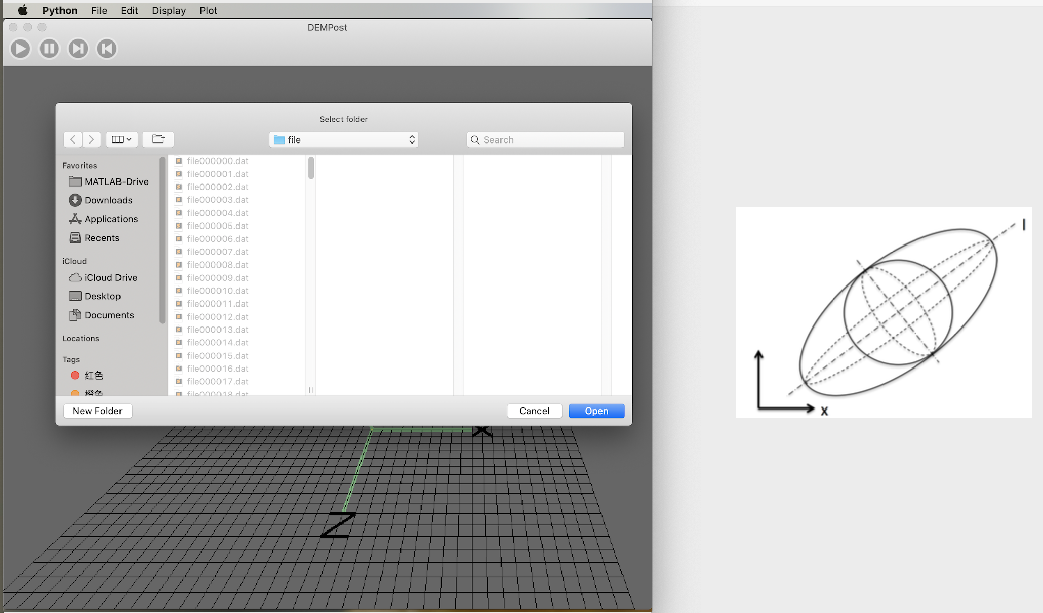
The data is calculated with DEM, which is stored inr the folder ForceeChain20170426, and the state data of the particles is in the subfolder /file. Each dat file in the catalog represents the flow of particles at a certain time, where each row represents a particle, a total of 21 columns. Information of data structure is explained in ReadMe.dat. In order to improve efficiency, load_data.py performs data cleaning, leaving only the following information of position, velocity and acceleration: (x_i, y_i, z_i, v{xi}, v{yi}, v{zi}, a{xi}, a{yi}, a{zi}) i=1, 2, 3,…. The list is passed to DEMPost.
- Parameter settings
After the file is determined, determine the object type of the model, select it in “File->Object” (Ctrl+O), use wxPython’s select list dialog box, “Particle Flow”, “Force Chain”, “Velocity”, “Acceleration” to select the four objects, and select the result that passed to DEMPost,
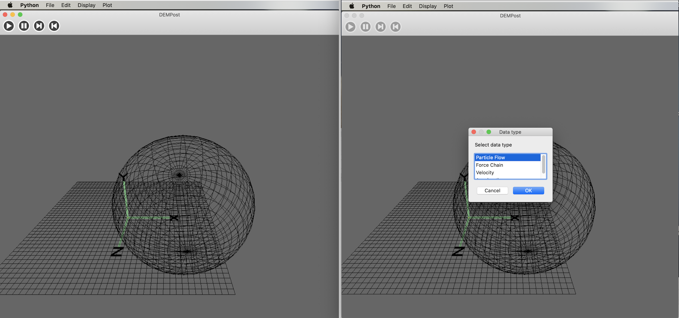
After the file is determined, determine the object type of the model, select it in “File->Object” (Ctrl+O), use wxPython’s select list dialog box, “Particle Flow”, “Force Chain”, “Velocity”, “Acceleration” to select the four objects, and select the result that passed to DEMPost.
To draw a particle flow model, you only need to use the coordinates, and pass the collection of individual particle coordinates to the combination class Particles.
Note that ParticleFlow also needs another parameter magnify, which represents the scaling factor of the particle coordinates, which is changed by “Edit->Parameter”(Ctrl+E). The process is as follows, click on the “Parameter” trigger text input dialog box, and the obtained user input is passed to the DEMPost canvas layer.
- Particle Flow visualization
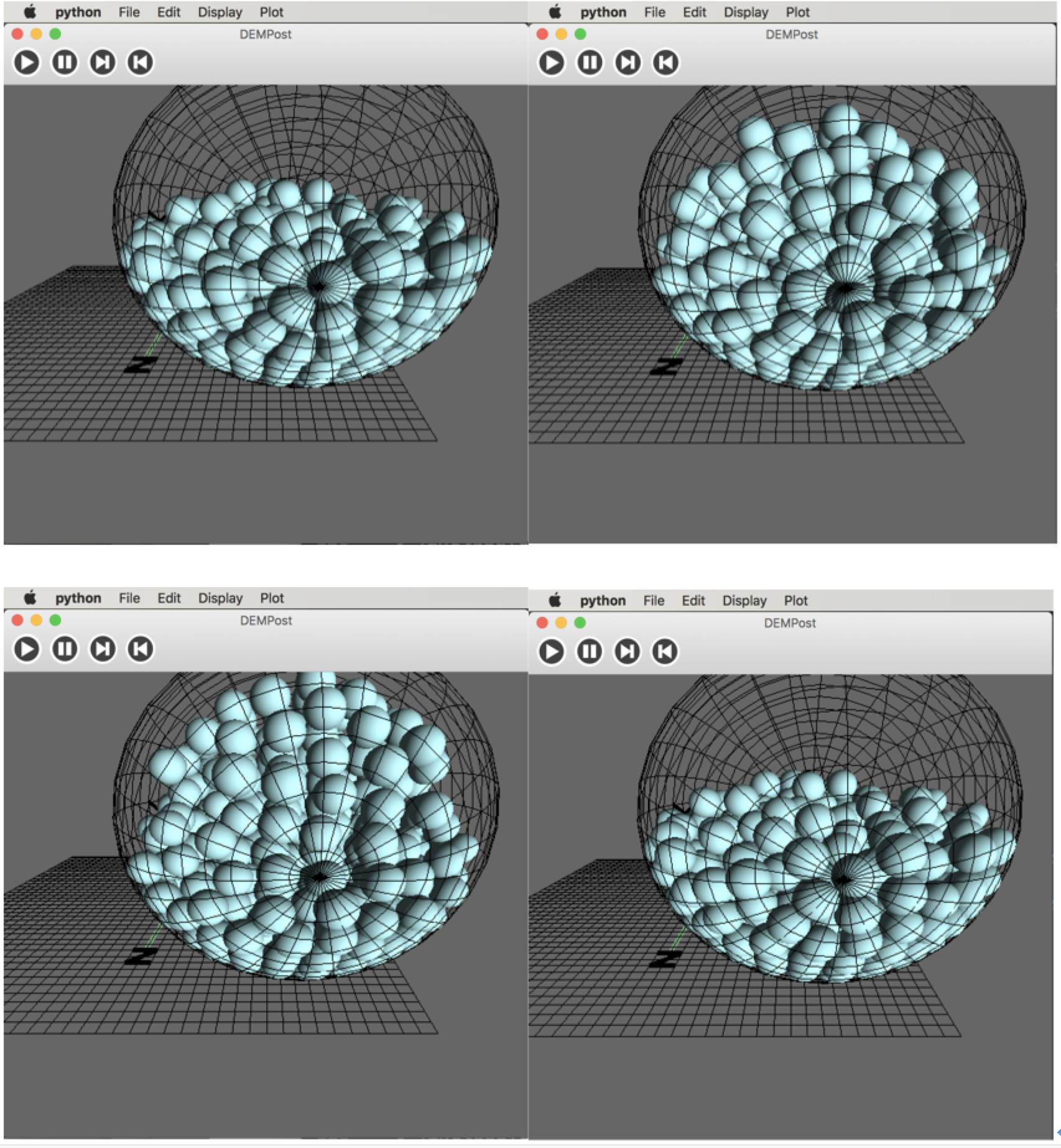
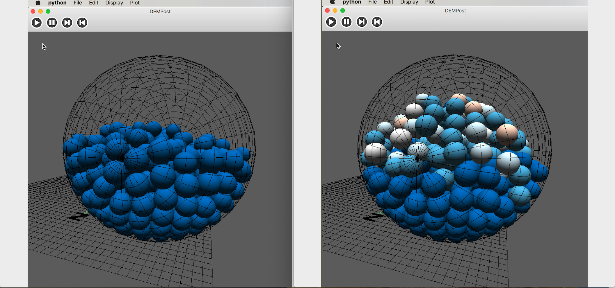
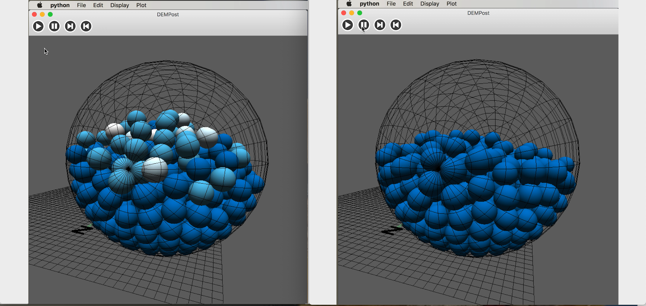
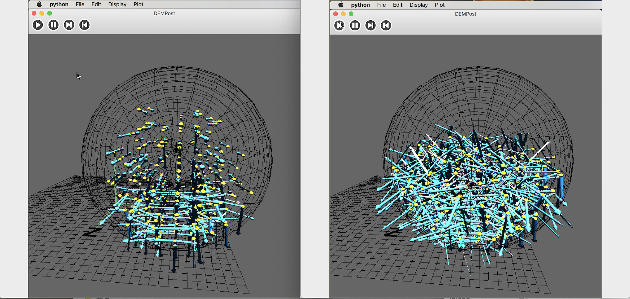
When the parameters are set, the particles can be drawn. In the menu bar, “Display->Show” (Ctrl+R), the implementation process is the same as the binding event mentioned in the previous two sections. The processed data is imported to the Particle stream datalist on DEMPost canvas to update canvas. Notice that there are no boundaries in the diagram, click “File->Import” Border to execute:
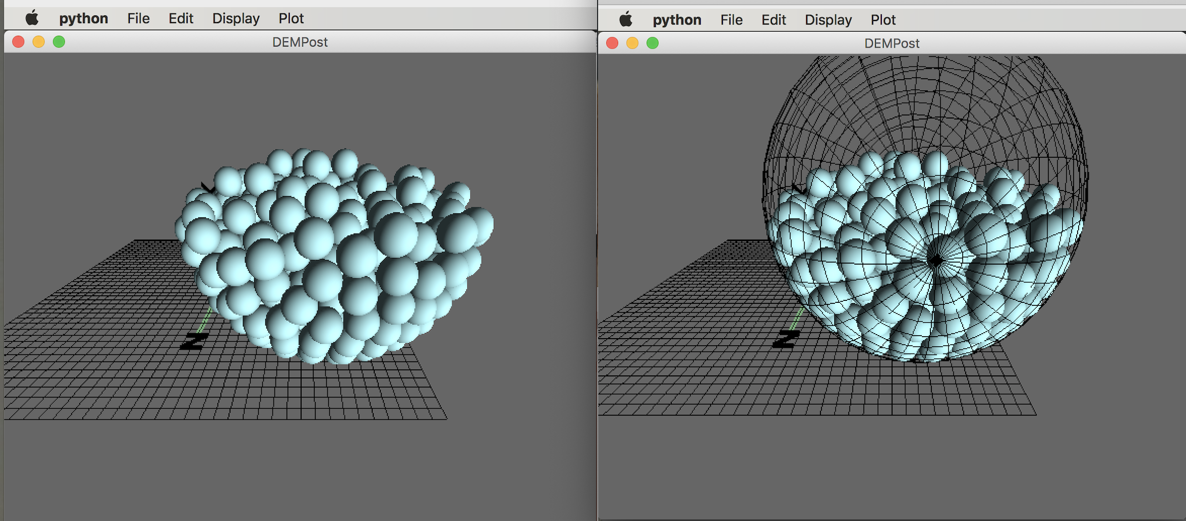
Use toolbar to control animation(Start, stop, next frame, previous frame). “Display->Clear(Ctrl+W)” clear the canvas and set the datalist, vellist, alist, linklist in the DEMPost canvas to an empty list to refresh the canvas.
- Velovity visualization
“File->Object”(Ctrl+O): select “Velocity” in the pop-up dialog box, the result is passed to the DEMPost canvas, and the datatype becomes”‘Velocity”.
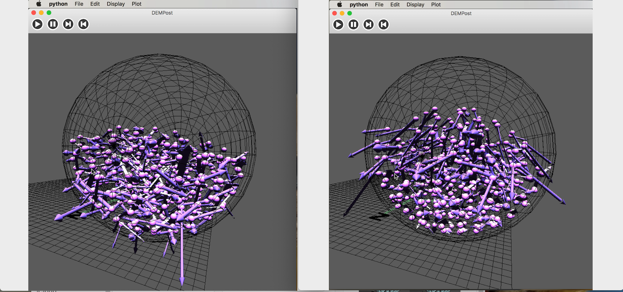
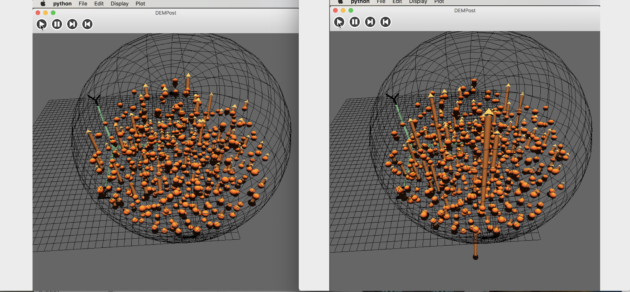
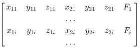
Since velocity is a vector, creating a composite class Vector in node.py. The particle velocity vector consists of particles and velocity vectors. It is an arrow shape consists of a Sphere and a Vector. The sphere is in the center of the corresponding particle, representing the position of the particle, Vector represents the velocity vector, the arrow points to the direction of the velocity vector, and the mode and velocity vector in proportion to the model,
1 | class Vector(HierarchicalNode): # the mode of the vector is 1, r is the radius |
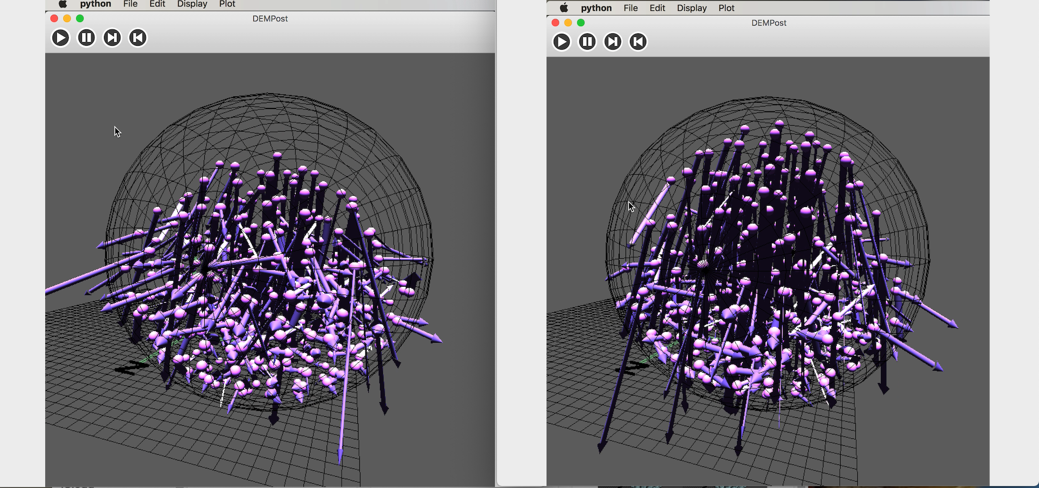
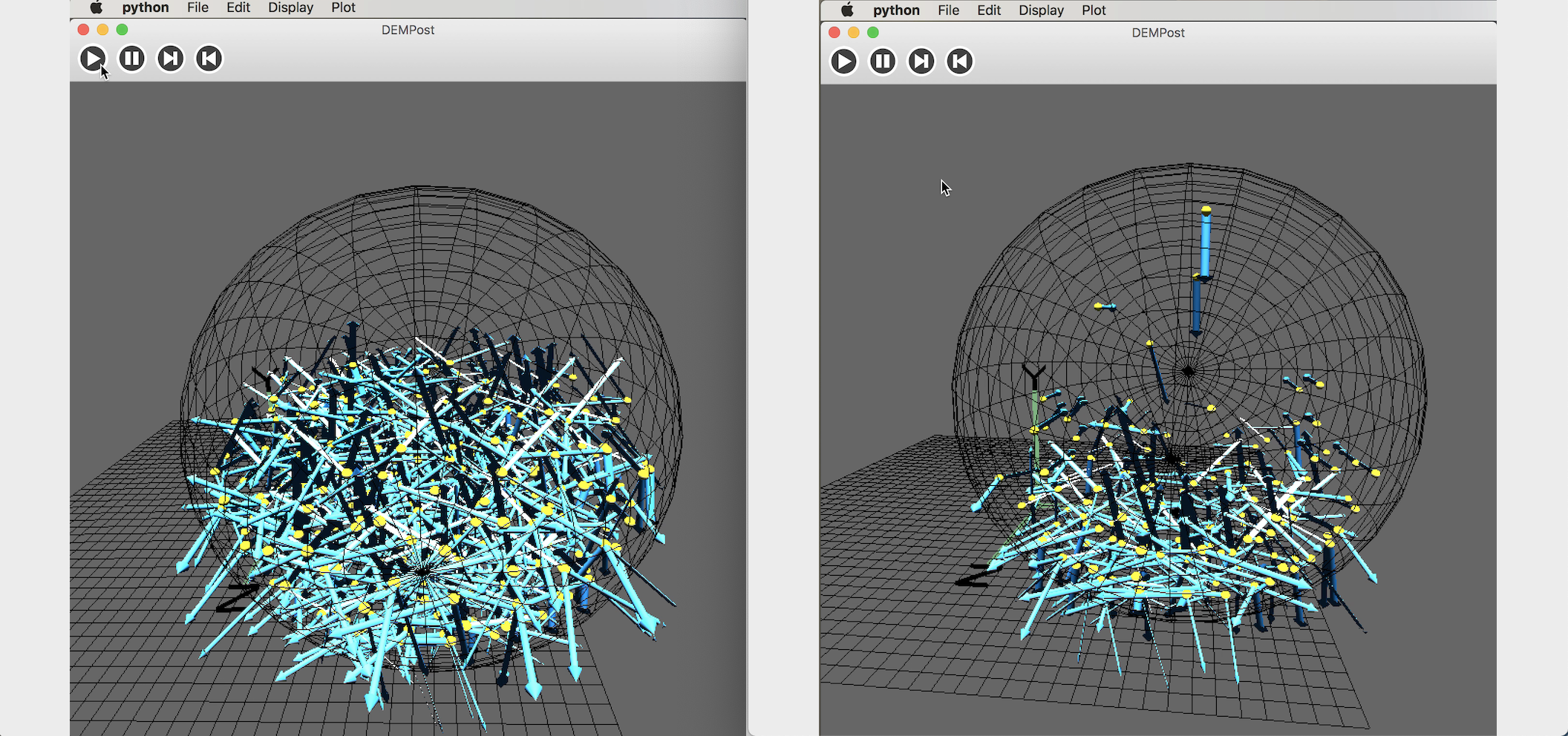
Like the particle stream, the value passed in DEMPost also represents the number of frames in the picture. It can be animated and controlled by the four buttons of the toolbar. It can be seen from the animation that when the particles are deposited at the bottom, the velocity is small. When some particles move above the boundary, the overall velocity becomes larger, the bottom velocity is upward, and the velocity is reversed after collision with the upper edge, and the particles are scattered around during the falling process. The velocity vector is radial. The velocity cloud map is used to represent the velocity,
- Acceleration visualization
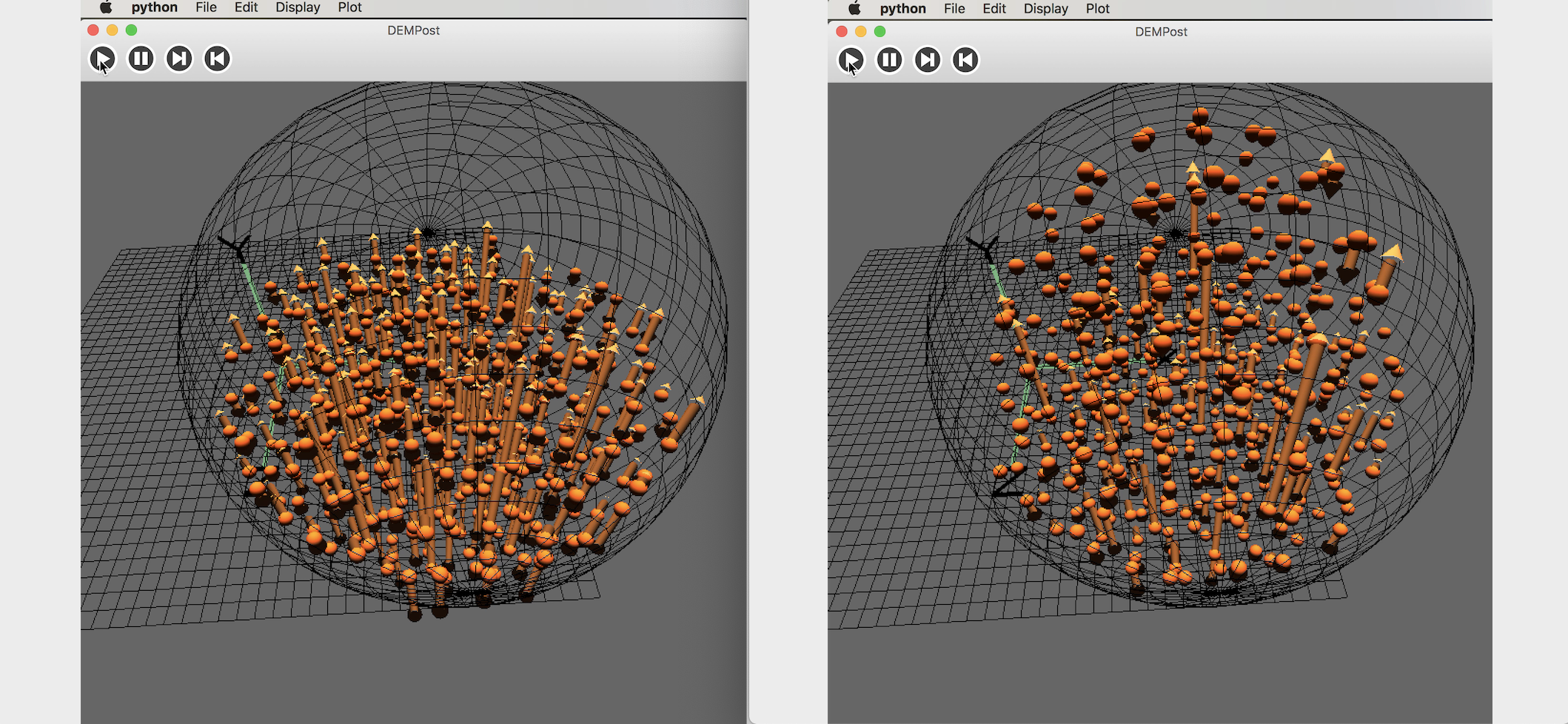
Acceleration vector diagram is similar to velocity. In order to distinguish, the author changed the color and adjusted to the appropriate parameter.
- Velocity and acceleration statistics
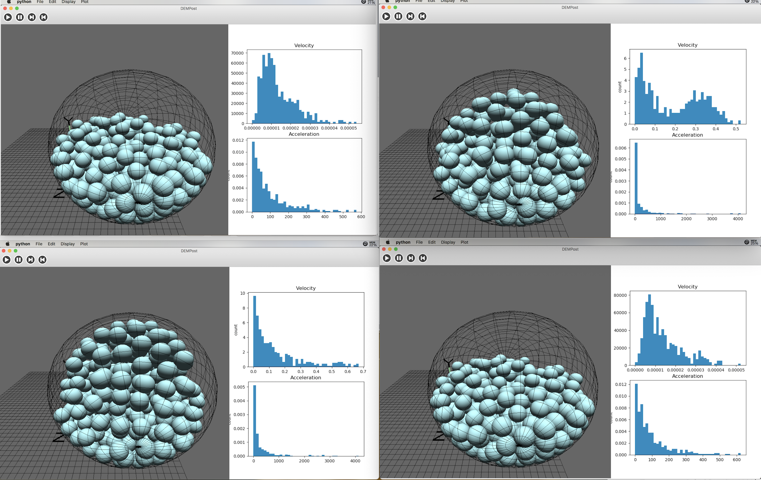
n order to observe the distribution of particle flow velocity and acceleration, DEMPost provides the function of displaying the histogram of variable distribution. Click “Display->Plot”
The object of statistics is the modulus of all velocities and accelerations, using the wxPython backend of matplotlib, creating the FigureCnavas object, embedding matplotlib into the GUI.
1 | from matplotlib.backends.backend_wxagg import FigureCanvasWxAgg as FigureCanvas |
- Force chain visualization
Force chain grids are often used in particle mechanics methods to represent the amount of force that exists between each pair of particles. DEMPost can also load and visualize a 3D force chain network. The force chain data/chains are also imported via File->Import(Ctrl+I). The data structure in each file is as follows,
Each row represents a force chain, the ith rows 1, 2, and 3 represent the xyz coordinates of the first and first particles in the i-th force chain in the force chain, and the fourth, fifth, and sixth columns represent the xyz coordinates of the second particle. Column 7 represents the magnitude of the force. In order to simplify the model, the force chain is regarded as a ManyVector arrow. The starting point is the first particle and the ending point is the second particle. The thickness of the wire is proportional to the force.
Background
- 3D Modeling and OpenGL
Computer-Aided Design (CAD) models the 3D world and creates and designs it on a computer. The key step in 3D modeling is rendering, which is to store and render as many and complex objects as possible, while keeping the rendering program less complex. Before rendering, you first need to create a window, because the graphics-driven manipulation is not enough, so you need to use a cross-platform image application interface OpenGL and OpenGL tool library GLUT to manage the window.
The render object of OpenGL is a polygon composed of vertices and normal vectors. Currently OpenGL has two branches: traditional OpenGL and modern OpengL. Traditional OpenGL provides a fixed pipeline. By adjusting global variables, developers can enable or disable some rendering features such as lighting, shading, and more. Next, OpenGL automatically renders the scene based on the features selected; modern OpenGL uses a programmable pipeline instead of a fixed pipeline, and developers only need to write shaders applets on graphics hardware such as GPUs. Traditional methods are relatively simple, and this article still uses traditional OpenGL programming. GLUT is a library bundled with OpenGL that creates an action window callbacks for the user interface. Due to the high requirements for frame management and user interface in this article, a complete library is required, thus wxPython interface is also used later.
In computer graphics, the basic elements are coordinate systems, points, vectors, and transformation matrices. The coordinate system consists of the origin and three basic vectors, denoted as the x-axis, y-axis, and z-axis; points in 3D coordinates can be represented as offsets to the origin in the x, y, and z directions. The vector represents the difference between the two points in the x-axis, y-axis, and z-axis directions; the transformation matrix can realize the conversion between coordinate systems. To convert a vector ν in one coordinate system to another, you can multiply a transformation matrix M:
v` = Mv
Common transformations include panning, zooming in/out, rotating, etc., which are called affine transformations. Figure below shows some of the transformations required from the physical object to the screen. The right half of the figure is the transformation of the object coordinate system (eye space) to the screen view (Viewort Space) can be implemented with OpenGL’s own functions; the inverse transformation from the object coordinate system to the screen view can be handled by gluPerspective, from Normalized device space, the conversion to the screen view can be processed by glViewport, and the two matrices are multiplied and stored as a GL PROJECTION matrix. The left half of the figure is implemented by the developer, defining a transformation matrix from the point in the model to the entity object as the model matrix, and then defining a transformation matrix from the entity object to the eye as the view matrix (view matrix ) view matrix, these two matrices are combined to get the ModelView matrix. The transformation of the 3D model The matrix is a four-dimensional matrix, because in the translation transformation, the fourth element determines whether the tuple is a point or a vector in space.
- Fundamental architecture of OpenGL
First, configure the lab environment and install python-opengl
1 | $ sudo apt−get install python−opengl |
Once installed, you can start building the viewer class DEMPost, which is implemented in viewer.py.
1 | class DEMPost(MyCanvasBase): |
Then rendering functions, update the buffer area,
1 | def OnDraw(self): |
Scene is the picture presented on the screen, the scene class is created in scene.py, the initialization code is as follows,
1 | class Scene(object): |
The objects rendered in the scene are all nodes in the scene. Next, define the node class and implement it in node.py.
1 | class Node(object): |
Next let’s define specific sphere class Sphere,
1 | class Primitive(Node): |
In addition to the spherical class, this paper also uses the cylindrical Cylinder and the conical Cone, which are all redefined in Node.py. Primitive is a class between a sphere class and a node class, and an important part of the model. Implementing pirmitive in primitive.py is called the glCallList method.All specific objects such as spheres, cubes, etc. are primitives, which can be rendered by OpenGL, glNewList(CALL LIST NUMBER, GL COMPILE) and glEndList() to indicate the beginning and end of a piece of code, and associate this code with one number. Therefore you can simply use glCallList (the associated number) to call this code.
1 | G_OBJ_SPHERE = 2 |
Where glCallList(G_OBJ_SPHERE) produces a sphere, it can also be combined into a model structure of other complex models, that is the composite node class HierarchicalNode, which is a subclass of Node.
1 | class HierarchicalNode(Node): |
Particle flow is also a combination class, which is a combination of many spherical classes.
1 | class ParticleFlow(HierarchicalNode): |
The three basic operations of translating, zooming and rotating is implemented by a change matrix in transformation.py.
In order to realize the user interaction with the scene, for example, to change the angle of view by dragging the mouse, to observe from different angles. Since the camera is fixed, we can only change the angle by moving the scene. Here I use the trackball algorithm to achieve. The principle of the trackball algorithm is that the origin of the world coordinate system is the center of the sphere. The scene is regarded as a ball with a sufficiently large radius, and the line of sight is unchanged. The angle of observation is changed by rotating the ball. In this article, to be brief, I use trackball defined in Glumpy directly. Use wget to download the trackball.py and store it in the working directory. The drag-to function updates the rotation matrix by taking the initial position of the mouse and the position of the mouse after the move, and stores it in the trackball.matrix of DEMPost to implement the scene. In order to rotate and update the ModelView.
1 | matrix.self.trackball.drag_to(self.mouse_loc[0], self.mouse_loc[1], dx, dy) |
- wxPython interface
wxPython is a cross-platform GUI toolkit for the Python language. It is an extension of Python, and also an open source software that supports Windows, MacOS and most Unix systems and can be installed directly using pip.
1 | $ pip install wxpython |
The GUI consists of a menu bar, a status bar, a toolbar, and a canvas. The first thing is to import wx Library, then create an application object and start the program.
1 | import wx |
I create a window canvasFrame with the size of 1000x776 and an initial position of (0, 100), which is the center of the left side of the screen. The menu bar is created in canvasFrame. The menu bar includes four drop-down menus, including File, Edit, Display and Plot. For each area of the management interface, the control panel is also required for initialization.
1 | self.panel = wx.Panel(self.frame, -1) |
Subsequent canvases are based on dashboards, such as visual area layers,
1 | class canvasFrame(wx.Frame): |
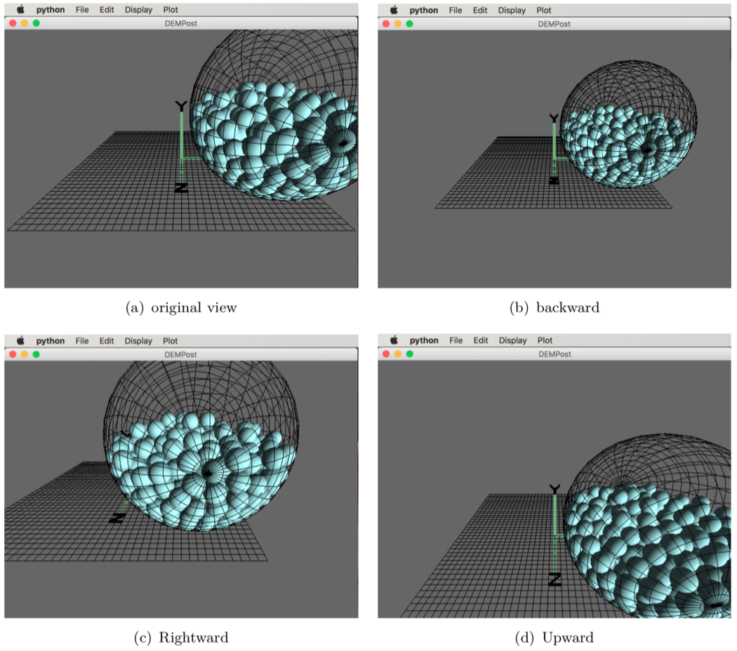
File->Quit (shortcut Ctrl+Q), “File” use wx.Menu() first to create menu filemenu, which defines a wx.MenuItem in this drop-down menu, self.Bind(wx.EVT MENU, self.OnQuit, id=3), event binder is used to associate the Quit function with the number 3 in the menu bar and the action to exit the window; In the drop-down menu Edit, the function Edit->Zoom in(Ctrl+’+’) /Zoom out(Ctrl+’- ‘) /Leftward /Righward /Upward /Downward respectively corresponds to the translational movement of the viewing angle in the direction of the front, back, left, and right, respectively. This is done through glTranslated(x, y, z) in the OpenGl.GL interface.
Then create a toolbar. There are four buttons on the toolbar, which are the animation start, animation pause, next frame and previous frame. The corresponding button icon exists in the working directory /Inc.
1 | toolbar = self.frame.CreateToolBar() |
Each frame is a scene representing a certain moment, and a time series is added to obtain a time state stream. You can animate the scenes at each moment. The implementation method of this paper is to give all the time data in the scene class DEMPost, number each frame; then use the self.timer function to calculate time When the picture at this moment is updated, the modified frame number is passed to DEMPost, The data corresponding to this frame is filtered out and the picture is re-rendered; the pause of the animation is to keep the time unchanged, and the timer is turned off. At this time, the frame number is unchanged, and the scene does not change; the previous frame/next frame button is to pass the number of the previous/next frame to DEMPost and re-rendering.
1 | def OnTimer(self, evt): |